- 본 게시글은 Factory Physics(3e, Wallace J. Hopp) 공부 정리글입니다.
- 개인적인 생각과, 책에 서술되지 않은 내용이 추가되었을 수 있습니다.
- 잘못된 이해에서 비롯된 오류는 지적해 주시면 감사하겠습니다.
Variability exists in all production systems and can have a significant impact on performance. In this chapter, we explore the concept of variability, the factors contributing to variability in individual processes, and methods for its calculation. Additionally, we examine variability within the flow when multiple processes are interconnected.
Process Time Variability
The key variable in Factory Physics is the effective process time(t_e) of a job at a workstation, denoted as "effective" because it encompasses the total time experienced by a job at a station(=actual working time, ex. 작업 시간 + 수리 시간)
Variability is quantified using variance, but absolute variability is less important than relative variability(분산은 평균에 값에 따라 상대적이기 때문, ex. 개미 키의 분산은 사람 키의 분산보단 당연히 작겠지?). A reasonable relative measure of the variability of a random variable is the coefficient of variation(CV), calculated as follows
c(=CV_, sigma(=standard deviation), t(=mean)
The following table is a table classifying the variability classes according to CV.
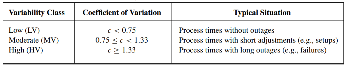
In many cases, t is more convenient to utilize the squared coefficient of variation (SCV):
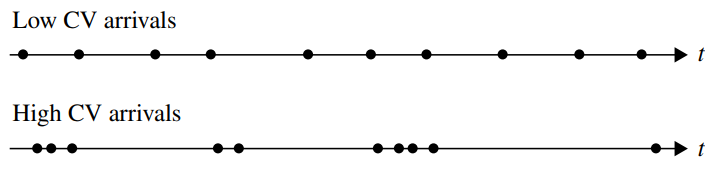
Picture belows tell us the relation to performance cases(Ch. 7)

The greater the variability in effective process times, the larger the average queue → The greater the variability, the longer the cycle time (by Little’s Law)
Causes of Variability
It is important to first understand the causes of variability. The most prevalent sources of variability in manufacturing environments are Natural variability, Random outages, Setups, Operator availability, Rework. 이제부터 각각을 살펴본다.
Understanding the causes of variability is crucial. The primary sources of variability in manufacturing environments are Natural variability, Random outages, Setups, Operator availability, and Rework. Let's examine each of these in turn.
Variability from Preemptive Outages (Random outages)
Natural variability refers to the inherent variation in process time, excluding random downtimes, setups, or other external influences. Even in tightly controlled processes, some degree of natural variability is always present.
A(=availability), m_f(=mean time to failure, MTTF), m_r(=mean time to repair, MTTR)
t_e(=effective mean process time), t_0(=natural process time)
(변동성과 고장을 고려한 실제 운용 시간을 의미)
r_e(= effective capacity (rate)), m(= # of machines)
c_e(=CV of effective process time)
The first term accounts for the natural variability in the process, while the second term represents variability resulting from random outages. Notably, this term persists even if the outages themselves (ex. repair times) are constant (ex. even if c_r = 0). However, the last term explicitly arises from the variability of repair times and would disappear if this variability were eliminated.
It's worth noting that both the second and third terms increase with mr for a fixed availability. Therefore, all else being equal, longer repair times induce more variability than shorter ones.
Conclusion: long, infrequent failures < shorter, more frequent ones < no failures

Variability from Nonpreemptive Outages (Setups)
N_s(=parts (or jobs) between setups, t_s(=mean of setup times)

Flow Variability
The discussion primarily addressed process time variability at individual workstations. However, variability at one station can influence other stations in a line through flow variability, which pertains to the transfer of jobs or parts. If an upstream workstation has highly variable process times, it will affect the variability in flows to downstream workstations. Thus, analyzing the impact of variability on the line necessitates characterizing the variability in flows.
r_a(=arrival rate), t_a(=mean time between arrivals)
c_a(=arrival CV)
In a serial production line, each workstation's output feeds into the next(all the output from workstation i becomes input to workstation i + 1). It's crucial that the departure rate from one workstation matches the arrival rate of the next to maintain continuous production flow.

u(=utilization), m(=# of identical machines)
The utilization (denoted by u) increases with both the arrival rate and the mean effective process time. An upper limit on utilization is one (=100%), indicating that the effective process times must satisfy a certain inequality.
Next, we will examine two scenarios: one where utilization is near 1, and the other where utilization is near 0. Subsequently, we will present a formula that integrates these two cases.
when u is close to one
When the utilization (u) is close to one, the station is alomst busy. Consequently, under such circumstances, the interdeparture times from the station closely resemble the process times. Thus, we would expect the departure CV to be the same as the process time CV (that is, c_d = c_e).
when u is close to zero
When the utilization (u) is close to zero, the station is very lightly loaded, it experiences extended waiting periods between job completions, as arrivals are infrequent. Given that process time constitutes a small fraction of the time between departures, interdeparture times closely resemble interarrival times. Thus, under these conditions we would expect the arrival and departure CVs to be the same (that is, c_d = c_a).
formula interpolating these two scenarios(when m=1, special case of general)
formula interpolating these two scenarios(when m>1, general case)
Obtaining information about the variability of interarrival times can be highly challenging, as such data is often not collected. However, variability in demand is frequently available. Fortunately, there exists a relationship between these two types of variability that allows us to infer one from the other.
u_n(= expected number of demands per period)
'공부 정리 > Factory Physics' 카테고리의 다른 글
| [Factory Physics] 8. Variability Basics (3) (0) | 2024.02.20 |
|---|---|
| [Factory Physics] 8. Variability Basics (2) (0) | 2024.02.20 |
| Kanban System(간판 시스템, 칸반 시스템) (0) | 2024.02.19 |
| [Factory Physics] 7. Basic Factory Dynamic (0) | 2024.02.05 |
| [Factory Physics] Chapter 6 (0) | 2024.02.03 |


